Your price-monitoring pipeline keeps flagging a dramatic competitor discount overnight. The product page hasn't changed. One parser has dropped a decimal separator, the historical baseline is distorted, and your alerting model is comparing valid prices against malformed values.
You patch the parser, but the problems don't end there. Review counts overwhelm ratings in your clustering model. Product titles that look identical still produce different hashes. A seller's updated name appears in some reports but not others because you've copied it into every observation.
Data normalization techniques solve different failures at different layers. Feature scaling changes numerical magnitude. Distribution transformations change shape or align batches. Unicode normalization makes equivalent text representations consistent. Database normalization separates facts according to their dependencies.
These methods aren't interchangeable. Scaling won't fix the wrong currency, and splitting tables won't repair an incorrectly parsed price. Start by preserving the raw value, validating its meaning, and identifying which downstream operation is failing.
For numerical transformations, the working pattern is consistent: fit on training or approved historical data, persist the fitted parameters, and transform incoming records without refitting them unnoticed. For text and schemas, version the rules so you can replay earlier records when your assumptions change.
1. Min-Max Scaling
Min-max scaling rescales a numerical feature to a fixed range, commonly between zero and one. It preserves relative spacing within the fitted range, making it useful when you want prices, ratings, and stock counts to contribute on comparable scales.
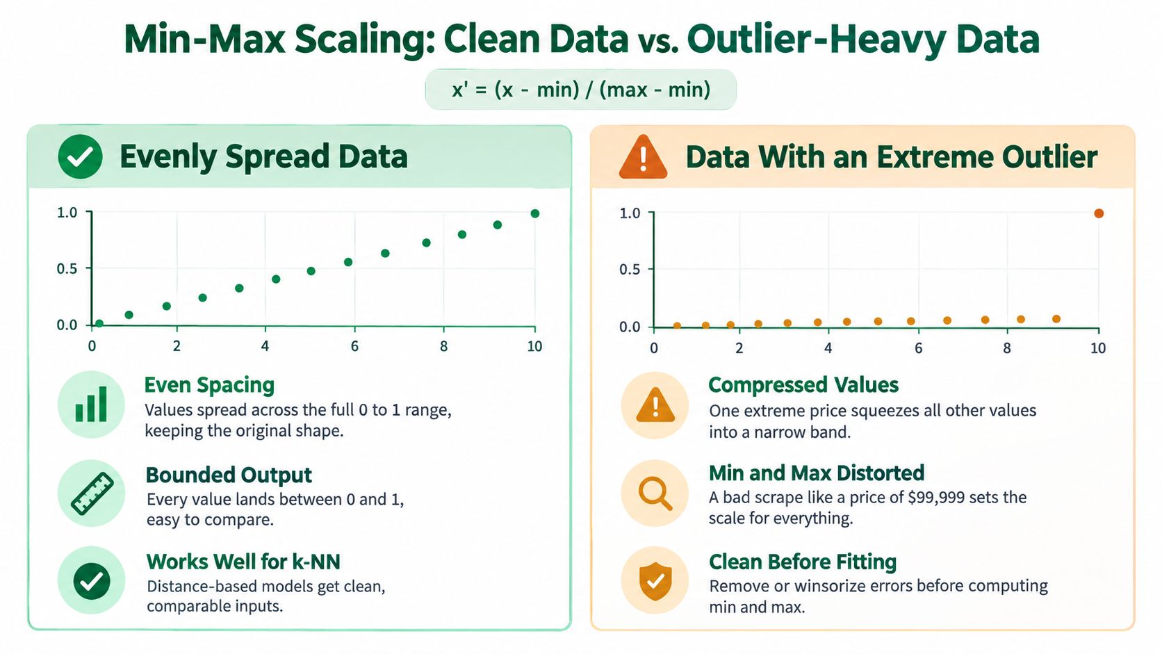
The formula is x_scaled = (x - minimum) / (maximum - minimum). Compute the minimum and maximum separately for each feature, not across an entire mixed-unit dataset.
Say you're clustering marketplace listings using price, review volume, and availability. Without scaling, review counts can dominate distance calculations just because their numerical values are larger. Min-max scaling removes that magnitude advantage, although you still need to decide whether those features deserve equal weight.
Keep Bad Values Out of the Fitted Range
An extreme parsing error stretches the range and compresses legitimate observations together. Apply data validation methods before fitting, including currency checks, numeric parsing checks, and category-specific plausibility rules.
In scikit-learn, initialize with scaler = MinMaxScaler(), call scaler.fit(X_train), then use scaler.transform(X_new). Put the scaler inside a Pipeline when cross-validating so each training fold gets its own fitted parameters.
- Handle constant features: A feature with no variation needs explicit handling because the mathematical denominator is zero.
- Track range violations: New observations can fall outside the fitted range. Flag them before deciding whether to clip.
- Preserve raw values: Clipping can hide genuine market changes as easily as malformed inputs.
Choose min-max scaling when bounded outputs matter and your reference range is trustworthy. Don't refit every scrape just to keep outputs inside the bounds, because that changes what yesterday's score means.
2. Z-Score Standardization
A price change can be ordinary for a volatile product category and exceptional for a stable one. Z-score standardization expresses a value relative to its baseline mean and standard deviation, rather than its original unit.
Use z = (x - mean) / standard_deviation. For a nonconstant fitted feature, this centers the reference data at zero and scales it to unit standard deviation.
This is useful before PCA, regularized linear models, and other scale-sensitive workflows. It doesn't require normally distributed inputs to perform the transformation, and it doesn't make a skewed feature normally distributed.
A standardized value describes distance from a fitted baseline. It isn't automatically an anomaly probability.
For competitor monitoring, calculate price changes after matching the same product, currency, package size, and seller context. Then fit category-specific baselines if categories behave differently. Otherwise, you're measuring incompatible observations against a shared average.
Use a Baseline That Matches Production
In scikit-learn, create scaler = StandardScaler(), fit it on the training split, and reuse it for validation and production. Persist the fitted means and scales alongside the model.
A rolling baseline can adapt to changing conditions, but it can also absorb a sustained parser failure until the failure looks normal. Keep an approved reference baseline for comparison, and schedule updates rather than recomputing parameters opportunistically.
The weak point is outlier sensitivity. Extreme values affect both the mean and standard deviation, potentially making genuine anomalies look less unusual. Validate malformed records first; for legitimate heavy tails, compare resilient scaling or a distribution transformation.
Choose alert thresholds against labeled examples and operational costs. Don't turn a conventional statistical cutoff into a production paging rule without checking false alerts, missed events, and category differences.
3. Robust Scaling
Scaling that resists outliers is a strong starting candidate for numerical scraped data with occasional extreme observations. Instead of the mean and standard deviation, it uses the median and interquartile range.
The formula is x_scaled = (x - median) / IQR, where IQR is the difference between the upper and lower quartiles. Because these statistics describe the middle of the distribution, isolated extremes have less influence on the fitted transformation.
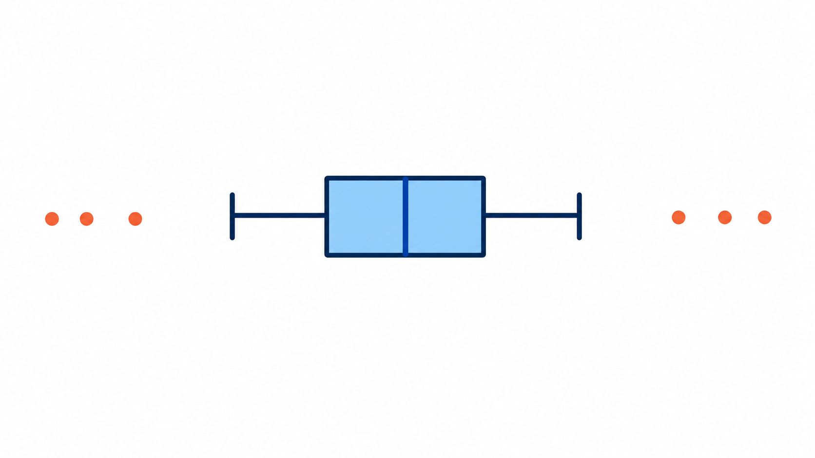
Consider marketplace prices containing ordinary listings, expensive bundles, and an occasional wrong-currency extraction. Resilient scaling keeps the ordinary listings distinguishable without letting the largest observation define the entire scale.
Resistance Isn't Validation
The bundle may be legitimate. The wrong-currency value isn't comparable. Outlier-resistant scaling reduces an extreme value's influence on fitted parameters; it doesn't correct its meaning or remove it from the output.
Use scaler = RobustScaler() in scikit-learn, then fit and transform through your training pipeline. Adjust quantile_range only when you have a distribution-specific reason, and record that setting with the fitted artifact.
- Validate first: Reject impossible values and separate incompatible currencies or units.
- Inspect sparse features: Review counts and stock signals can have a zero interquartile range when many observations are identical.
- Define a fallback: For degenerate features, drop the feature, use a documented alternate scale, or retain a categorical indicator.
Avoid adding an arbitrary tiny denominator without inspection. That can turn modest differences into enormous transformed values.
Choose resilient scaling when extremes are expected but central differences still matter. Compare it with a log transform when the entire distribution is heavily skewed, rather than assuming every large observation is contamination.
4. Log Transformation
Follower counts, review volumes, and page views often have a long right tail. A log transformation compresses large values more strongly than small values, making relative differences easier to model without requiring an identical distribution across features.
For positive values, use y = log(x). For nonnegative counts that include zero, y = log(1 + x) is convenient; NumPy implements this as np.log1p(x).
Suppose you're comparing engagement signals from scraped creator profiles. A raw follower-count feature can overwhelm smaller accounts numerically, while a logarithmic feature lets the model work with proportional differences more naturally.
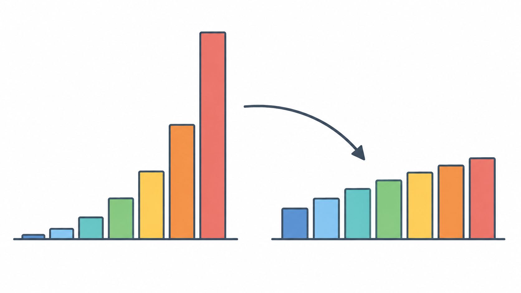
The transformed distribution may become less skewed, but it won't necessarily become symmetric or Gaussian. Compare histograms and tail behavior before and after transformation instead of treating the function call as proof of improvement.
Keep Units and Inversion Explicit
A logarithm changes interpretation. A model trained on log-transformed outcomes predicts on the transformed scale unless you explicitly invert its output.
Use np.expm1(y) to invert log1p. If you're estimating expected values, recognize that back-transforming a mean prediction doesn't generally recover the original-scale conditional mean.
Practical rule: Use a log transform to manage meaningful multiplicative variation, not to make a broken parser's output look less extreme.
Don't apply ordinary logarithms to signed price changes or negative balances. A signed-log mapping is possible, but it has different semantics and should be documented.
Choose log transformation for nonnegative, right-skewed features where proportional differences matter. It's deterministic and doesn't need fitted distribution parameters, although any subsequent scaler still must be fitted on training data only.
5. Yeo-Johnson Power Transformation
Price-change features contain decreases, increases, and unchanged observations. Ordinary logarithms don't handle that signed domain, so Yeo-Johnson is useful when you want a fitted power transformation that accepts negative values and zero.
It estimates a shape parameter, lambda, for each feature. The transformation uses separate branches for nonnegative and negative inputs, with logarithmic limiting cases.
The Transformation in Practice
For nonnegative inputs, the main branch is ((x + 1)^lambda - 1) / lambda, with log(x + 1) when lambda is zero. For negative inputs, the main branch is -((1 - x)^(2 - lambda) - 1) / (2 - lambda), with -log(1 - x) when lambda is two.
You rarely need to implement those branches yourself. In scikit-learn, use transformer = PowerTransformer(method='yeo-johnson', standardize=True), fit it on X_train, and transform held-out observations with the same object.
For a competitor-pricing model, compare transformed price-change features with the original signed changes. Keep whichever representation improves held-out performance and calibration, not whichever produces the prettiest histogram.
- Persist the fitted object: Store lambda values and any standardization parameters with the model.
- Check mixed populations: A feature combining unrelated categories may stay multimodal after transformation.
- Inspect tails: Maximum-likelihood fitting doesn't make the method immune to malformed extremes.
Yeo-Johnson isn't a general requirement for regression. Linear regression doesn't require every predictor to be normally distributed, and tree-based models often gain little from a monotonic feature transformation.
Choose it when skewness is causing a measurable modeling problem and signed values rule out a straightforward log transform. Refit deliberately, because changing lambda changes the representation consumed by downstream models.
6. Quantile Normalization
Quantile normalization aligns distributions across samples or batches by replacing rank positions with shared reference values. Unlike feature scaling, it deliberately removes differences in distribution shape.
In the classic procedure, sort each comparable sample, average the values at each rank, and assign those rank averages back to the original observations. Handle ties explicitly so identical input values don't receive arbitrary different outputs.
A plausible use case is repeated extraction of the same reference panel through different collection routes. If technical collection effects change a derived score's distribution, alignment may help you compare the panel consistently.
Don't normalize away a market difference just because it makes the box plots line up.
Ratings from different marketplaces aren't automatically interchangeable, and regional search results can differ for legitimate reasons. Aligning those distributions without a defensible reference can erase the signal you intended to measure.
Separate Batch Alignment From Feature Mapping
Classic cross-sample quantile normalization isn't the same operation as scikit-learn's QuantileTransformer. The latter fits an empirical distribution for each feature and maps observations to a selected target distribution.
For a reference-based feature mapping, the implementation might begin with mapper = QuantileTransformer(output_distribution='normal'). Fit it on training data only, and understand that mapping tails can distort numerical distances.
- Define comparable batches: Match the population, measurement, and collection conditions before alignment.
- Freeze a reference: Don't let every incoming batch redefine historical scores.
- Retain originals: Analysts need raw values to distinguish collection artifacts from real changes.
Choose quantile normalization only when distribution differences are known nuisance effects. Inspect density plots, rank preservation, and downstream decisions after transformation. If you can't explain why the distributions should match, don't force them to.
7. Unicode Text Normalization
A product title can look identical in your dashboard while differing at the code-point level. Unicode normalization reconciles equivalent character representations before matching, indexing, or hashing.
NFC composes canonically equivalent sequences where possible; NFD decomposes them. NFKC and NFKD also apply compatibility mappings, which can remove distinctions such as character width or presentation variants.
For catalog deduplication, start with NFC on extracted titles and names. Keep the original text alongside the normalized value so you can inspect unexpected matches.

Build Separate Display and Matching Values
In Python, normalize with unicodedata.normalize('NFC', text) after importing unicodedata. For a field where whitespace differences are irrelevant, " ".join(normalized.split()) collapses whitespace and trims the ends.
That whitespace operation is a separate cleaning decision, not part of Unicode normalization. So are case folding, accent removal, punctuation mapping, and transliteration.
Use a dedicated matching key if you need more aggressive transformations. Applying unicodedata.normalize('NFKC', text).casefold() can be appropriate for some search fields, but compatibility mappings may collapse distinctions that matter in identifiers or technical text.
- Normalize before hashing: Otherwise equivalent representations can still produce separate records.
- Keep field-specific rules: Product descriptions, source code, personal names, and SKUs shouldn't share an indiscriminate cleanup function.
- Test collisions: Review cases where distinct raw strings produce the same matching key.
Good data parsing practices establish what a field means before text normalization changes its representation. Unicode normalization won't repair incorrectly decoded bytes, translate names, or reliably identify visually confusable characters.
Choose NFC for conservative canonical consistency. Use compatibility normalization only where you've explicitly decided that the affected distinctions don't matter.
8. Database Normalization (1NF to 3NF)
Database normalization organizes facts so that updates don't leave contradictory copies. For scraped commerce data, that usually means separating product identity, seller identity, listings, and time-stamped observations.
First normal form requires atomic values without repeating groups. Second normal form removes partial dependencies on candidate keys, while third normal form addresses transitive dependencies between non-key attributes.
Say a listing observation contains a seller identifier, seller name, product identifier, current price, and collection timestamp. Store the seller's current attributes separately from the observation, unless you intentionally need the name as observed historically.
Separate Identity From Observation
Use stable identifiers scoped to their source, and enforce foreign keys and uniqueness constraints. Treat URLs cautiously as natural keys because redirects, tracking parameters, and URL changes can complicate identity.
Keep prices and availability as observations with explicit timestamps and collection context. Your choice of CSV versus JSON affects interchange and nesting, but neither format guarantees a normalized relational model.
Normalization isn't automatically a performance penalty: an IMDb and PostgreSQL experimental study found that moving from first to second normal form reduced on-disk database size by 10% and reduced energy consumption per transaction by 74% under its tested conditions.
A controlled PostgreSQL benchmark also found that aggressive denormalization reduced median read performance by 1.95–2.91× at small scale factors in its tested row-store configuration. Wider rows and extra reads can outweigh the benefit of avoiding joins.
Keep a normalized source of truth, then optimize measured read paths. Inspect query plans and indexes before materializing repeated joins, and define freshness and reconciliation rules for duplicated outputs.
For a visual explanation of table decomposition, use this walkthrough.
Watch the video on YouTubeHow the 8 data normalization techniques differ at a glance
| Item | Best For | Outlier Handling | Output Range | Stored State Needed |
|---|---|---|---|---|
| Min-Max Scaling | Scaling features to a fixed range | Sensitive; extremes compress other values | Usually 0 to 1 | Fitted minimum and maximum |
| Z-Score Standardization | Centering features for statistical and gradient-based models | Preserves outliers; mean and standard deviation are sensitive | Unbounded; often around -3 to 3 | Fitted mean and standard deviation |
| Robust Scaling | Scaling skewed data with outliers | Median and IQR resist extremes; outliers remain | Unbounded | Fitted median and IQR |
| Log Transformation | Compressing large values and reducing right skew | Compresses extremes without removing them | Unbounded; depends on input and log variant | Transform choice, such as log or log1p |
| Yeo-Johnson Power Transformation | Making positive, zero, and negative data more symmetric | Can reduce skew; behavior depends on fitted parameter | Unbounded | Fitted lambda parameter |
| Quantile Normalization | Aligning distributions across samples or batches | Maps values to a shared reference distribution | Values from the reference distribution | Reference quantile distribution |
| Unicode Text Normalization | Consistent text matching, search, and deduplication | Not applicable to numeric outliers | Normalized text representation | Chosen Unicode form |
| Database Normalization (1NF to 3NF) | Organizing relational data to reduce redundancy | Not applicable to numeric outliers | Relational tables organized by normal forms | Schema, keys, and relationships |
Match the Method to the Failure You Are Seeing
Start with the symptom, not the technique. If an extreme value distorts your fitted scales, compare outlier-resistant scaling after validating the record. If legitimate counts have a long right tail, test a log transformation before adding a more complex fitted method.
When batches disagree for technical reasons, evaluate quantile normalization against a stable reference. When duplicates survive visual inspection, normalize Unicode before generating matching keys. When updates leave contradictory copies of the same fact, fix the table dependencies rather than adding another cleanup query.
Several data normalization techniques can belong in the same pipeline, but they need different contracts. A product title might receive NFC normalization, a review-count feature might receive log1p, and the underlying observations might live in normalized relational tables.
Make Every Transformation Replayable
Keep the raw source value, canonical value, source timestamp, transformation version, and validation status. Recent AI pipeline engineering guidance treats normalization as the place to establish a stable downstream shape while accommodating upstream API drift.
That matters when a website silently changes a price field from text to a nested object, or starts using an unavailable marker where it previously omitted the field. Don't collapse absent, unavailable, invalid, and not-applicable values into the same default unless their business meaning is genuinely identical.
- Version fitted artifacts: Save scalers, reference distributions, feature order, and model compatibility together.
- Monitor incoming records: Track validation failures, missingness changes, range violations, and unexpected field shapes.
- Quarantine ambiguous inputs: Preserve enough context to repair and replay them instead of coercing them into plausible-looking values.
For selectively denormalized reporting outputs, define who owns refreshes and how stale values are detected. Adobe's normalization guidance supports treating denormalization as a targeted read-path optimization rather than abandoning a normalized foundation.
Upstream, reduce avoidable structural variation at collection. Scrappey's AI Extraction lets you describe fields and receive JSON in exactly the structure you define, without maintaining selectors. That gives normalization a consistent input structure, but you should still validate currencies, units, identity, and missing-value meaning before trusting the extracted values.
Pick a failing downstream operation, build a representative test set, and compare the simplest suitable transformation against the current pipeline. Promote the change only when it improves the decision you care about and you can reproduce the result from preserved inputs.
Scrappey offers web data access and AI-powered extraction into a user-defined JSON structure, giving your normalization pipeline a more consistent starting point. Visit Scrappey to define the fields for a sample product or search-results page, then validate the extracted records before applying your chosen transformations.